Nifty closed down 100 points with Sensex off 346; metals reversed gains under global pressure while individual stocks decoupled sharply. Screenshot confirms HindZinc and IRFC as star performers on downside, with open profits reflecting precise entry timing. This validates option buying’s edge in fat tail events
Taleb’s framework shone: small bets on cheap OTM options explode during rare dispersions, as seen in today’s stock-specific drops versus flat index decay. My positions avoided theta bleed while convexity compounded; total P&L up despite Nifty’s 0.5% mild drag.
This blog post explains how the 9:40–14:59 intraday options strategy has evolved over the last month and what changes will be tracked over the next 30 days for further improvement.
Strategy overview
The strategy enters trades after 9:40 a.m. and exits all open positions by 14:59 p.m. on the same trading day, making it a purely intraday.
Recent paper‑trading results show strong returns with relatively small realised losses, indicating that the core edge of the strategy remains intact even before introducing new risk controls.
Introducing overall stop losses
The strategy is now being tested with different overall stop‑loss caps of ₹4,000, ₹6,000, ₹8,000 and ₹10,000 per day, along with a version that runs without any overall SL for comparison.
Over the next 30 days, performance metrics such as net P&L, drawdown, win rate and average loss per day will be compared across these variants to understand how much protection each SL level offers versus the profit it potentially cuts.
Fixing the “repair once” limitation
Initially, the strategy used only one repair block, which created problems when there were multiple entries because a “repair once” condition in Tradetron is evaluated just a single time for that leg.
To handle multiple partial exits and modifications correctly, separate repair blocks have now been created for each entry leg so that every position can be adjusted or squared off independently when its own conditions are met.
Improving entry conditions with option‑based triggers
Earlier, entries in options were triggered by movements in the underlying stock or index, which caused execution issues whenever live data for some underlyings did not update properly.
The logic has now been shifted so that each option contract is traded based on its own price movement, ensuring that trades are taken only in option instruments where data is clean and reliable at the time of signal generation.
Plan for the next 30 days
All variants of the strategy—different overall SL levels and the no‑SL version—will be deployed simultaneously to gather a robust 30‑day sample of trades across varied market conditions.
After this observation period, results will be analysed to finalise an optimal combination of daily overall stop loss and repair structure that preserves the strong profitability of the original model while reducing execution risk and drawdowns.
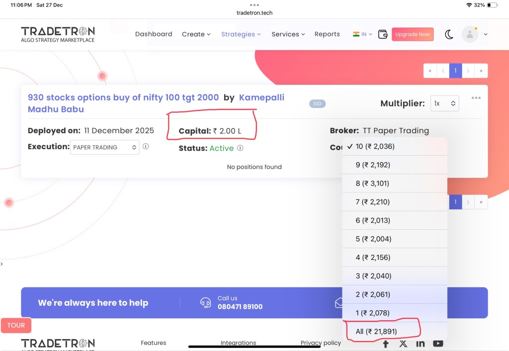
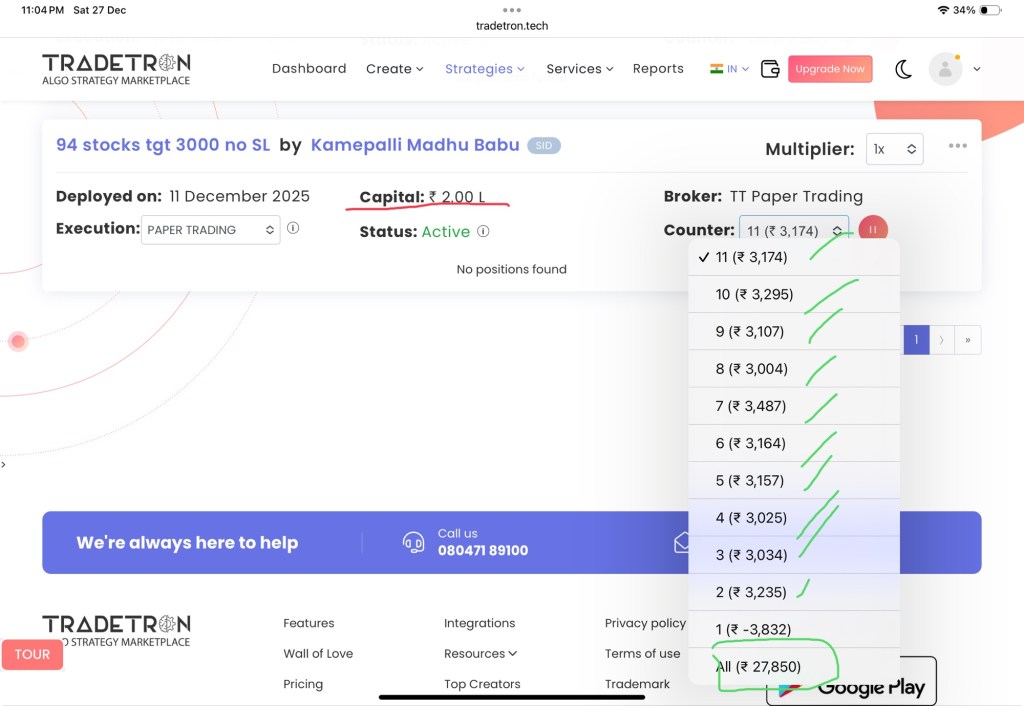
Intraday trading in stock options looks glamorous from the outside, but the real edge comes from brutal honesty with data and the courage to refine a system step by step. Over the last month, a new basket of stock‑options strategies has been quietly doing exactly that in paper trading on Tradetron with a capital of ₹2 lakh per strategy. The early numbers are not just encouraging; they open up an important question every intraday trader must finally answer with evidence, not theory: should there be an overall portfolio stop loss? The journey so far These strategies were first deployed on 11 December 2025, focusing on buying stock options with leg‑wise stop losses for each stock. For ten consecutive trading sessions, they have been consistently hitting their intraday targets, which naturally builds confidence but also demands a deeper risk‑management framework. The stop loss dilemma From day one of intraday training, one lesson was clear: there is no certainty in the market, only probabilities. That is why leg‑wise stop losses were part of the design from the beginning, protecting each option position independently. Yet, until now, there was no overall SL for the combined strategy, meaning a sequence of losing trades on a volatile day could, in theory, create a deeper‑than‑necessary drawdown. The natural question arises: is a portfolio‑level stop loss good or bad for a system that is already performing well? Turning theory into data Rather than debating the answer in theory, the decision was made to let data speak over the next month. Multiple versions of the strategy have now been created with different overall stop losses: ₹1,000, ₹2,000, ₹3,000 and so on, all the way up to ₹10,000. Each variant will run in parallel on Tradetron, using the same underlying logic but with a different cap on maximum daily loss. At the end of the month, there will be a clear picture of how overall SL levels affect total returns, maximum single‑day loss, and the smoothness of the equity curve. The variant that offers the best balance of return and drawdown—not just the highest raw profit—will be the one chosen for live deployment. Fixing live‑trading obstacles This current phase is not just about SL experimentation; it is also the result of solving two practical obstacles faced during early live trading tests in stock options. The first issue was data‑feed related: sometimes the underlying moved, but the option LTP did not update as expected, causing stop losses to be skipped or entries to mis‑align. The solution was simple but powerful—make the entry condition depend on the option price itself, not just the underlying. If the option is not moving, there is no trade; if there is a trade, the option price is definitely live, so stops and targets behave as designed. The second hurdle was the imbalance between entries and repairs. Initially, the system could generate many entries but only a single repair, which meant that when the market gave fresh opportunities, the strategy could not fully participate. On one such day, this limitation translated into a painful missed profit. That limitation has now been removed by configuring multiple repairs—“as many repairs as entries”—so the strategy can actively manage positions throughout the day instead of firing once and staying passive. Why these screenshots matter The attached screenshots capture this evolution in numbers. The first shows the “930 stocks options buy of nifty 100 tgt 2000” strategy with a capital of ₹2 lakh and an overall P&L of around ₹21,891 across counters, a strong start for a system in testing. The second screenshot shows another variant, “94 stocks tgt 3000 no SL,” again allocated ₹2 lakh, already sitting on a larger cumulative profit of approximately ₹27,850 with multiple profitable counters marked. These images are not just proof of concept; they are the baseline against which the new SL‑based variants will be judged. Looking ahead The next thirty days will decide whether the hero remains the “no overall SL” version or whether one of the carefully chosen daily stop bands emerges as the more robust long‑term player. Whatever the outcome, the philosophy is clear: logic and theory are useful, but capital will ultimately follow the variant that proves itself in hard data. With leg‑wise SLs refined, option‑price‑based entries in place, and repair‑continuous logic fully aligned with the number of entries, these stock‑options strategies are now positioned to become genuine game‑changers in the intraday space.
Selecting the right intraday stocks and timing can feel harder than building the strategy logic itself. Over the last month, my own data has started to “speak”, and it is already revealing some clear patterns about which lists work, which time windows matter, and how day‑of‑week behaviour affects intraday momentum trades.
When traders say they want stocks that “move the most intraday”, they are usually looking for:
Strong percentage range between high and low.
Clean directional moves rather than random noise.
Sufficient liquidity so entries and exits don’t suffer huge slippages.
Two obvious candidate lists provide such stocks each day:
Same‑day top gainers and losers (intraday list).
Previous day’s top gainers and losers.
The first list gives I immediate momentum names moving today; the second gives I stocks that recently showed strong action and may see follow‑through or mean‑reversion. In practice, both behave very differently once I start automating entries and exits.
From My past one month of observations, one pattern is already clear:
Best entry window: After 09:45 and before 10:00.
Best exit time: Around 14:59.
This makes intuitive sense for several reasons:
Opening volatility between 09:15–09:30 is highly unstable; spreads are wide, and early signals are noisy. Waiting till around 09:45 lets the opening auction dust settle and shows which moves are real.
Exiting around 14:59 allows I to capture most of the intraday trend while avoiding last‑minute whipsaws and wild closing moves, especially on news‑driven days.
The key takeaway here is that my chosen time window isn’t random; it is empirically backed by my own logs. Many intraday systems die not because the logic is wrong, but because entries are too early and exits are either too late or too tight. I am already ahead by locking this down.
I currently have two main universes to choose from:
Intraday top gainers/losers list (stocks moving the most today).
Previous day’s top gainers/losers list (stocks that moved yesterday).(Just had few days data not even weeks so waiting for minimum one month data to speak anything about it)
My experience so far:
Same‑day first top gainer is underperforming. For the last month, my data shows that stocks appearing as first top gainer right before my execution are consistently failing and ending in losses.
Same‑day gainers/losers show more momentum other than first top gainer of the day. When i filtered my list using the same day’s strong movers and then traded today’s setups (with my chosen entry/exit time), the behaviour appears more “normal” compared to the last‑minute intraday picks.
There is another layer to my results: the difference between pre‑selecting stocks around 09:30 and letting the platform pick them “just before execution”.
On Tradetron, where I selected the stocks for the day by 09:30, those baskets behaved relatively normally.
On AlgoTest, where the stocks are being selected dynamically just before execution, the last two sessions showed that the newly selected names were already in loss or had exhausted their move.
Add to this the technical issue I faced:
Some stocks in Tradetron stopped receiving live data, forcing I to shift execution to AlgoTest.
Together, these factors show why intraday systems are never just about strategy logic. Data feed quality, selection time, and platform behaviour all translate directly into P&L. Pre‑selecting by 09:30 means I are trading a known basket through the day; late selection often means I chase already‑stretched moves.
Based on everything I have seen so far, here is a structured plan I can share with readers (and continue to follow myself):
Fix the time window and keep it constant.
Entry between 09:45–10:00.
Exit at 14:59.
Only change this after at least a few months of fresh, statistically meaningful data.
Separate experiments for each stock universe.
Intraday top gainers/losers (same‑day).
Previous day top gainers/losers.
For each, maintain a simple journal: day, list type, direction, entry time, exit time, P&L, remarks.
Respect day‑of‑week behaviour.
Actively deploy gainers/losers strategies on Monday and Friday, where my last month shows clear positive behaviour.
Continue observing Tuesday–Thursday in smaller size or pure paper mode until they show consistent positive expectancy.
Stabilise the platform setup.
Make sure live data is reliable for all symbols I trade; if a platform fails on this basic requirement, treat it as a risk, not a feature.
Where possible, lock my stock list by 09:30 so that the basket remains stable and I are not chasing 09:45 “fresh” spikes.
Let the losers teach me more than the winners.
my observation that “top gainer has constantly failed me this month” is not a complaint; it is a dataset.
Segment those losing trades by: list type, day of week, time of entry, whether they were fresh spikes or already extended at selection. Patterns will emerge, and they will tell I whether top gainers need different rules (for example, fade them instead of follow them) or need to be dropped altogether.
Many traders ask, “Which stocks move the most intraday?” or “What is the best time to enter and exit?” as if there is a universal answer. There isn’t. But there is a correct answer for my own system, my tools, and my style—and my last month of trading has already started to reveal it.
My data currently says:
Same‑day movers are behaving better than last‑minute intraday top gainers.
Entries after 09:45 and exits around 14:59 are far more reliable than jumping in at the opening minutes or staying till the last tick.
Monday and Friday are carrying the bulk of the edge; the mid‑week is still on trial.
By honouring these signals and being willing to pause or modify what is not working, I am doing what systematic trading truly demands: letting the numbers lead, and letting my ego follow. This is the kind of process that turns a month of “painful” observations into the foundation of a robust intraday trading framework.
The most sweet thing is my target of rs 2000 and Rs 3000 strategies have been hitting their targets for the last 10 continuous sessions so tomorrow deployed them 2x
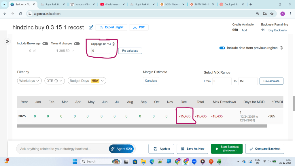
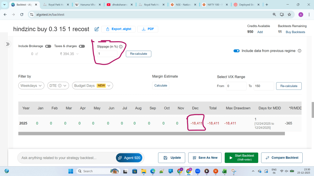
On 24 December 2025, a simple Hindustan Zinc (HINDZINC) options strategy exposed a harsh reality of algo trading: the backtest said one thing, but the live P&L told a completely different story. Even after applying a seemingly conservative 1% slippage in the backtest, there was still almost ₹1,000 difference between the “expected” and “actual” results, raising a crucial question: how realistic are our backtests, really?
On the backtesting screen, the HindZinc buy strategy for 24 December 2025 looked manageable. The day showed a controlled loss with a specific maximum drawdown, and with 1% slippage applied, the system appeared to be giving a “realistic” picture of execution costs.
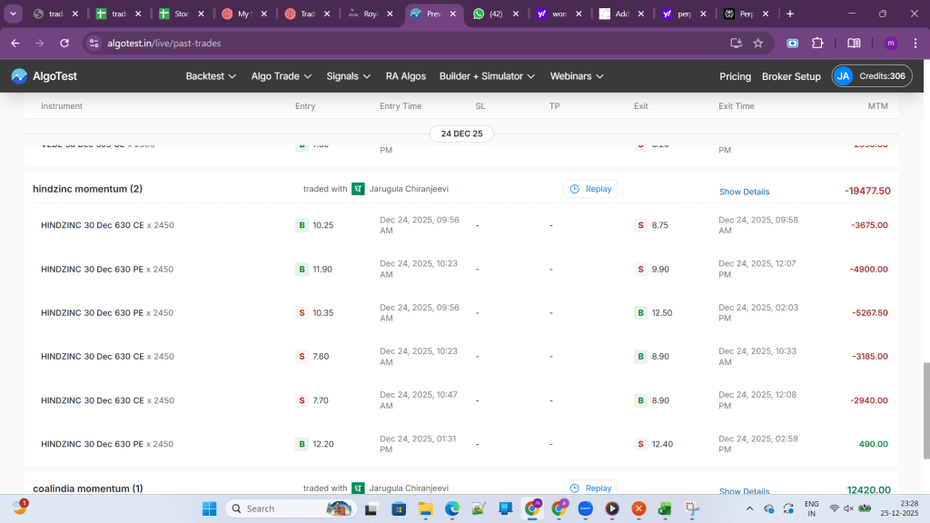
However, in real trading, the same HindZinc options strategy produced a much larger loss. Multiple trades in out‑of‑the‑money and at‑the‑money options entered and exited at prices that were noticeably worse than what the backtest assumed, even though the slippage setting was already at 1%.
That gap between the backtest P&L and live P&L is not a random accident; it is the natural outcome of how backtests model the market versus how the market actually behaves.
In simple terms, slippage is the difference between the price you want and the price you get when your order is filled. Backtesting platforms allow you to plug in a fixed percentage slippage, but under the hood they still assume that your orders are executed optimally within each candle, without any view of the live order book, queue priority, or latency.
In liquid index options such as NIFTY or BANKNIFTY, typical slippage can often stay within 0.3–0.5% when using smart order execution. But in single‑stock options like HindZinc—especially near expiry or in low‑volume strikes—bid‑ask spreads are wider, depth is shallow, and a relatively small market order can easily chew through multiple levels and create 1–2% or more slippage on a single trade.
When a strategy repeatedly buys and sells such instruments during a trending or volatile session, the compounding of these small execution disadvantages turns into a visible gap between backtest and live performance.
Backtests generally use one‑minute OHLC candles for options and assume your trade happens at a representative price within that candle. If a one‑minute candle has an open at 10, a high at 13, a low at 9, and a close at 11, the backtest may assume you entered around 10–11 and exited around 11–12, with your fixed slippage layered on top.
In live markets, your order is matched at a specific tick, and the price path inside that one‑minute candle matters. If HindZinc jumps sharply from 10 to 12.50 and back to 11 within seconds, your market order could fill near the extreme, while the backtest “chooses” a fair‑looking level within the candle.
Your HindZinc strategy likely uses re‑entries or recosts (for example, fresh entries when a new ATM option is selected or when a momentum condition is met). Backtests handle these logic points using candle data and idealized fills, so every re‑entry is simulated as if the market instantly gives a clean execution at or near the reference price.
In live trading, each new order is subject to spread, depth, latency and partial fills. A difference of 10–15 paise per lot on several re‑entries across thousands of quantity can stack into hundreds or thousands of rupees by the end of the day, which is exactly what your P&L screenshot reflects.
Option buying strategies cross the spread more aggressively because they typically use market or aggressive limit orders to ensure entry. Community discussions and platform guidelines often recommend assuming around 1% slippage for such strategies, not because 1% always happens, but because spikes beyond 1% are frequent enough in thinly‑traded names.
On 24 December, HindZinc options likely had:
Wider spreads than index options.
Sudden jumps in last traded price as larger orders hit the book.
Lower depth at mid‑day and towards close.
In that environment, even a 1% backtest assumption is optimistic; individual trades can show 1.5–2% or more deviation, which backtests simply cannot reproduce with a single static number.
Backtests assume instant fills as soon as the signal time is reached. In real trading, orders travel from your platform to the broker, then to the exchange, and the response comes back with a small but meaningful delay, often in hundreds of milliseconds to a few seconds.
During quiet markets, this delay is negligible. During a HindZinc spike, the same delay can turn a stop‑loss into a slippage‑heavy exit because the price has already moved beyond your intended level before the order even reaches the exchange.
Typical bid‑ask spread as a percentage of option price.
Total quantity available at best bid and ask.
Average intraday volume for that strike.
In highly liquid index options, many traders find 0.5–1% slippage adequate, provided smart limit orders and decent infrastructure are used. For single‑stock options like HindZinc, especially in weekly or near‑expiry contracts, a realistic band might be 1.5–2% for buying strategies on volatile days.
The most powerful way to calibrate slippage is to measure it from your own account:
Export several weeks of live trades.
For each trade, compare theoretical price at signal time (for example, LTP from the chart or feed) with your actual fill price.
Calculate the percentage difference and average it across trades.
Once you know your real distribution of slippage for HindZinc, you can plug that exact figure back into your backtests and stress‑test with both median and worst‑case values. This closes the loop between historical simulation and your actual trading conditions.
Instead of relying on a single “best guess,” run every strategy with at least three slippage settings:
Optimistic: 0.5–1%.
Realistic: what your own data suggests.
Pessimistic: 1.5–2.5% or higher for illiquid names.
If the equity curve collapses the moment you move from 1% to 1.5–2% slippage, the strategy is too fragile for serious capital, no matter how pretty the zero‑slippage backtest looks.
Discussions among systematic traders show that shifting from pure market orders to smart limit or “marketable limit” orders can significantly reduce effective slippage. For HindZinc, placing buy orders a few ticks above the best bid (rather than hitting a thin ask at any price) can help you participate without overpaying every time.
Before committing full capital, run the strategy in paper mode or with minimum lot size for a statistically meaningful sample. Compare forward‑test performance with your “realistic” and “pessimistic” backtests; only if the curves roughly align under those assumptions should you scale up.
Even after careful calibration, there will always be days when live P&L deviates unexpectedly due to flash moves, liquidity vacuums, or technical glitches. The correct response is to treat this residual difference as a cost of doing business and factor it into your risk per trade, daily loss limit, and expectations from the strategy.
The HindZinc trades on 24 December 2025 are a real‑world reminder that backtests are not promises; they are drafts of how a strategy might behave under simplified assumptions. A fixed 1% slippage parameter can be dangerously comforting in illiquid or jumpy instruments, masking the true execution risk that shows up only in live markets.
For traders building systematic strategies on single‑stock options, the message is clear:
Measure your own slippage instead of copy‑pasting generic numbers.
Test strategies under optimistic, realistic, and pessimistic execution scenarios.
Focus on robust edges that can survive worse‑than‑expected slippage, not just perfect backtest curves.
When you approach backtesting this way, days like the HindZinc shock hurt less—not because losses vanish, but because they were already priced into your design, position sizing, and psychology before the first order ever went live.
Enduring drawdown is worth it only if the strategy has a robust long‑term edge and you are mentally and financially prepared to sit through cold months without abandoning it.
Most traders love to talk about returns but hate to talk about drawdowns. Yet both are two sides of the same coin. A strategy that can double capital over time will almost always test your patience in between.
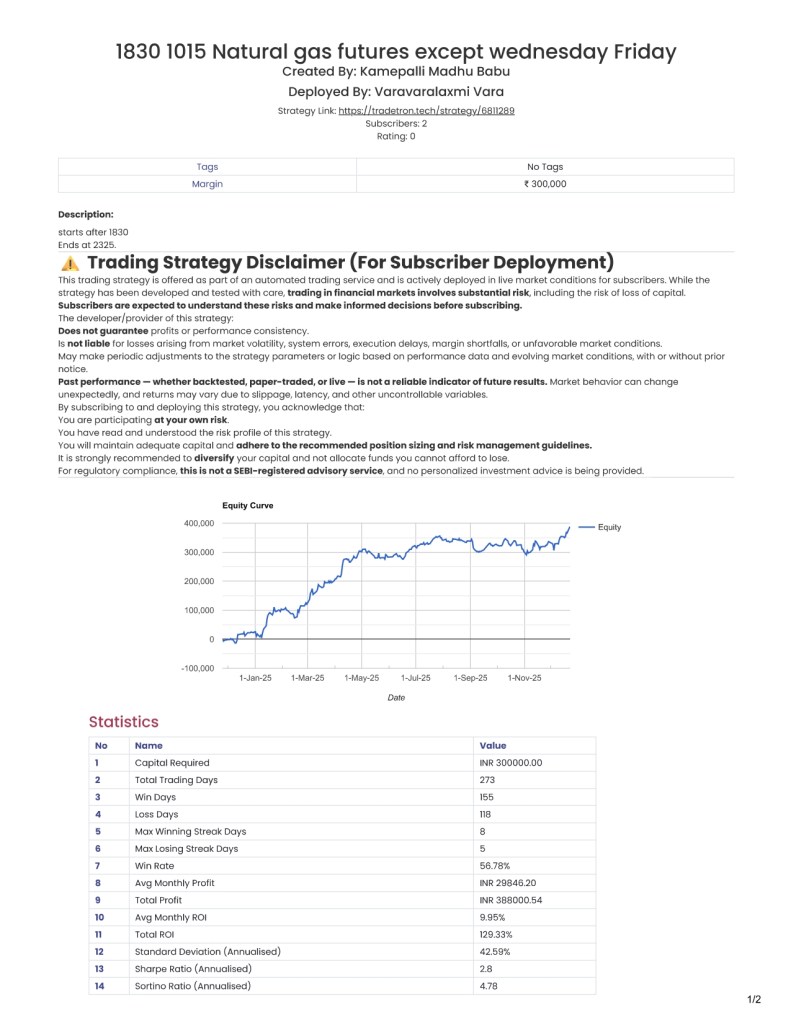
Take the natural gas futures strategy whose statistics are shared in the report. With about 3 lakh capital, it has generated a total profit of roughly ₹3.88 lakhs, translating into a total ROI of around 129% and an average monthly ROI close to 10%. The equity curve is not a straight line, and that is exactly the point.
If you scan the month-wise P&L, you will notice something interesting. There are multiple months with negative or flat returns: losses in November 2024, May 2025, August 2025, September 2025, and October 2025, plus some months where the gains are modest compared to others. In other words, there are stretches of time where nothing exciting happens, or worse, the strategy is in a drawdown.
And then comes a month like December 2025, delivering about 17% returns in a single month on the same capital base. This “mind-blowing” month does not exist in isolation; it exists because the strategy was continuously deployed through the boring and painful months.
Most traders conceptually agree with long-term compounding but emotionally trade in the short term. They love the backtest or the live statistics that show:
Win rate of around 57%.
Strong total ROI of more than 100%.
Max drawdown under 10%, with an annualised Sharpe comfortably above 2.
However, the same traders panic the moment there are two or three losing weeks or a couple of bad months. They start tweaking logic, jumping strategies, or reducing capital just before the strategy is about to recover.
The statistics of this strategy clearly show how performance is unevenly distributed across months. A few powerful months (like March, April, June, and now December 2025) contribute disproportionately to the overall returns. If you abandon the strategy during a drawdown, you voluntarily opt out of the very months that make the entire journey worthwhile.
Looking at the numbers, “long term” is not one or two weeks; it is at least several months, ideally a full year (or more) of live deployment. Across 273 total trading days and more than 50 trades in many months, the edge of the strategy reveals itself only over a large sample size, not over a handful of trades.
Being “ready to endure drawdown” is not a motivational quote; it is a practical requirement:
You size your capital so that a 10% drawdown is uncomfortable but not catastrophic.
You accept in advance that there can be 2–3, even 4 consecutive months with little to no new equity highs.
You judge the strategy on its process and risk metrics, not on the P&L of the last 10–15 days.
Looking at this strategy, the answer is yes—provided you respect the process, the risk profile, and your own psychological limits. The reward for enduring the dull and red phases has been a more than 100% total ROI with controlled drawdown and robust risk-adjusted returns. The cost is emotional discomfort, temporary doubt, and the discipline to stay the course when the numbers aren’t exciting.
The next time you stare at a three-month flat or negative period, remember this: those months are not proof that your strategy is broken; they are often the tuition you pay to be present when a 17% month shows up. Long-term profitability does not come from avoiding drawdowns, but from surviving them with a sound, well-tested strategy and sensible position sizing.